Tumbling, Appendix II: Getting Formal

24 Jul 2011 Pre-Ramble

The problem with what I've described previously is it's all a bit fuzzy - it's based on flow diagrams and vague descriptions, it was informal, and lacked precision. Mathematics, however, likes to have ideas clarified, by transforming them into precise, but somewhat impenetrable, collections of symbols. And who am I to argue with maths?

Having found PlosOne and arXiv, which offer open-access to academic papers, I've come across a few papers - some related to subjects in my blogs - that have grabbed my interest. And usually I'll skim over them, then download for reading 'at a later date'. But even just skimming, I have started to picked up a few tricks

Being as this is just an informal blog, there's nothing wrong with being informal. Nonetheless, there's no harm in a little practice. So this is an attempt to reintroduce the model (derived previously) as a formal set of equations. It should be noted, though, that none of this changes or nullifies what was previously written. It simply sets it out in a more precise - albeit cryptic looking - way.

Consider this fair warning of what's to follow.


But First...

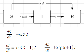
For completeness, I wanted to redefine the model as a compartmental one. For what it's worth. It would look and work something like this
In this case, alpha roughly reflects the average number of followers a user has, and beta the approximate average reblog rate. (gamma = 1 - beta). As discussed previously, this model isn't really sufficient. But it's nice to look at for comparison.

In fact, the exposed state (E) isn't strictly necessary in this case (more on that below). It's more of a placeholder, included for clarity. You can actually rework the model to get rid of it; in which case, it looks like this
Here's an example of what the output might look like (N=10,000, alpha=0.001, beta=0.14),
With the compartmental form of the model, because the variables - such as the reblog rate - are constant, the behaviour across multiple simulations is uniform.

In fact, for the same initial conditions, the results will always be the same. By comparison, the behaviour of the model previously outlined can vary wildly between multiple simulations, run with the same initial conditions.

You could modify it - maybe make the variables, literally, variable - but since we already have a perfectly good model, it's not really worth bothering.


Preamble

First of all, these are difference equations - as opposed to the differential forms used above. This is because we're working in discrete steps (rather than continuous), and because the equations aren't, strictly speaking, time dependent.

Second, for this formal approach, we're working in matrices. It's just easier that way.

Now. For the simulated model, I created the network at random, as I went. This was on the assumption that it would be computationally faster. But for formality, we suppose that the entire network is either known, or else generated prior to simulation.

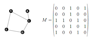
At any rate, it works like this - define a matrix, M, with entries,
This is, essentially, a table of ones and zeros that represents some (arbitrary) network of connections - i.e. who follows who.

As an example, in the below, the matrix on the right represents the graph on the left,
From this, we can calculate things like: the number of people a user, i, follows, and the number of people user i is followed by (respectively) as
That is, in the left case, sum along the i-th row, and in the right, sum down the i-th column.

Next, we define column matrices for each of the possible states. So, for example, the susceptibility matrix, S, has entries
That is, if user i is susceptible at time n, then this will be indicated by a one in the i-th row of that state matrix. Otherwise its value is zero.

We can then define an operator to calculate the number of people in that given state as
Essentially, this counts the number of ones in whichever state matrix. Which leads to the equation
Which basically says that the sum of the number of people in each state equals the total population size.  Or in other words, that everyone in the population has to be in one of the three states.

Finally, we define a function, sigma, that looks like this,
This is the function for threshold testing, described previously. In essence, it takes a matrix of the users' thresholds, t, and their assessments of a given post, A(p), and returns a matrix of ones and zeros representing whether or not each user will 'reblog' that post.


The Model

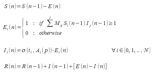
So now, we can define our set of equations. Brace yourself,
The typical initial conditions will be,
In theory, this model shouldn't be significantly different from the one previously outlined - though, admittedly, I haven't tested this assumption.

Ultimately, the behaviour of the system depends on the matrices M, t, and A(p). And if these are predefined and fixed, then the behaviour will be the same over multiple simulations. But if these are newly generated (at random) for each simulation, then the behaviour will be variable, as before.

In this case, E(n) is really more a function, upon which the other equations depend, rather than a state in and off itself. In particular, no-one exists in that state for any longer than it takes for them to be redistributed into their proper state (for that iteration). This is similar to the redundancy of the E state in the compartmental model above, except that this time it's not so easily written out.

And that's basically it.


Oatzy.


[Hoping I didn't make any mistakes in my own model.]